A Machine Learning Approach to Target Gain & Stop Loss – Learn When to Exit a Position

Stop-loss and target gain methods were originated by professional day traders looking to exploit short-term price displacements. In recent years, with a wider adoption of algorithmic trading, rule-based exit conditions expanded in scope for all investment styles, including long-term strategies.
Recent price volatility has caught many investors by surprise, and theory has been quickly replaced by soul searching focusing on one question: “How much pain am I willing to endure?”
Many who consider themselves sophisticated investors look to place an arbitrary fixed percent stop-loss based on one’s age, financial health, and investment goals. However one overriding factor remains, the investor’s personal pain tolerance. In theory, placing a fixed stop loss sounds like a good and easy approach to implement. In reality however, most investors will be sorely disappointed or consider themselves very “unlucky” when they either exit prematurely (leaving money on the table) or when they have to endure substantial losses.
Placing an overly conservative stop-loss can close positions prematurely, and can also lead to missing out on potential gains. Conversely, employing an overly relaxed exit condition will result in substantial losses, and often will leave the investor even more frustrated when the closed position reverses back into gains which will no longer be realized.
Truth be told, exit condition science is somewhat complicated and requires a careful algorithmic approach in which risk levels are assessed dynamically both at the individual asset and overall market levels.
At Neuravest, we’ve done extensive research on the science of exit conditions and this blog is meant to explain why most exit condition implementations fail. Further we will discuss how deep reinforcement learning can be used effectively for an algorithmic exit strategy.
Why placing a static stop loss and target gain doesn’t work?
Let’s take for example the following scenario: You’ve entered a position at a price per share of $10.00. Assessing the stock’s trading range for a one-month outlook (look forward) using one-year history yields a distribution of returns with a mean at 0%.

Image #0: Distribution of returns.
Translating to our position, we expect that during the normal course of business, the stock will oscillate between $9 and $11.
Statistically speaking, using a simplified Monte Carlo distribution model and discounting the market, transaction costs, and slippage (more on that a bit later), if we put a target gain at the expected peak of $11 and a stop loss at the trough of $9, we will have an equal chance to exit with gains or losses of 10%.

Image #1: Statistically we have an equal chance of exiting with profits (denoted in green) or losses (denoted in red).
A naive approach would be the following: We can reduce our threshold for target gain by half to +5%. This increases the probability of reaching the target gain threshold substantially. For the sake of argument, assume that the probability of reaching the +10% threshold is half that of reaching the +5% threshold. In reality, the aforementioned assumption is optimistic as returns are approximately normally distributed, see Image #0. In other words, in a perfect world if the stock oscillates evenly between the +10 and -10%, It will be twice as likely to gain 5 than to lose 10%.
In reality, even this idealized scenario won’t turn profitable.
Consider the chart below:

Image #2: We start with $10 and apply a sequence of 2 wins of 5% each followed by a single loss of 10%. After a few iterations our $10 decayed into $9.54.
The reason we have actually lost money is due to a concept called exponential decay. As it takes more “effort” (n + e) % to make up for a n% loss.

Image #3: It takes more than 11.11% to recover a 10% loss.
In reality, this decay is even more pronounced since we incur transaction costs and slippage each time we enter and exit a position. In addition, the market conditions and volatility continuously change. For this reason a more dynamic exit criteria model is needed.
Making Stop Loss and Target Gains Dynamic
Let’s take a look at some approaches to determine exit conditions. We will start with a naive static approach and progressively add dynamism and complexity as we attempt to be completely data-driven with no human discretion.

Image #4: Visualization of applying a Fixed Threshold of +/- 2%.
The naive “Fixed Threshold” approach is to assign upper and lower thresholds at the time of entering a position. The dollar value of these thresholds above and below the current price is based on an arbitrarily chosen “acceptable” percent change. In Image #4, this value is chosen to be +/- 2%. Once determined, the upper and lower bounds remain static until one of them is crossed, thereby exiting the position.

Image #5: Visualization of applying a Trailing Threshold of +/- 2%.
The “Trailing Threshold” approach adds a slight layer of complexity. Once calculated, the dollar value of the upper and lower thresholds are reapplied on a rolling basis according to price. While the distance between the upper and lower bounds is static, the value of these bounds is adjusted day to day.

Image #6: Visualization of applying an ATR Threshold.
The “ATR Threshold” approach is to assign upper and lower thresholds at the time of entering a position according to the stock’s idiosyncratic volatility expressed by its ATR (average true range) calculated over a recent lookback period. The bounds are therefore decided from historical price action information and not determined arbitrarily. Once computed, the upper and lower thresholds remain static until one of them is crossed.

Image #7: Visualization of applying an ATR Trailing Threshold.
The “ATR Trailing Threshold” approach adds a slight layer of complexity. Again, the bounds are calculated in a data-driven manner according to historical price information. Once calculated, the upper and lower thresholds are reapplied on a roll forward basis each time a new high is reached. While the distance between the upper and lower bounds is static, the value of these bounds is adjusted to protect the gains already incurred.

Image #8: Visualization of applying a Dynamic ATR Threshold.
The “Dynamic ATR Threshold” approach adds one more layer of complexity. Bounds are computed according to ATR over a historical lookback period. These bounds are static and set based on price for the day on which they are calculated. After N days, the thresholds are recomputed according to ATR over a historical lookback period, and the process repeats.

Image #9: Visualization of applying a Dynamic ATR Trailing Threshold.
The “Dynamic ATR Trailing Threshold” increases complexity further. Bounds are determined according to ATR calculated over a historical lookback period. Once computed, the upper and lower thresholds are reapplied on a roll forward basis according to price for N days. On day N+1, thresholds are recalculated according to ATR over a historical lookback period, and the process repeats.

Image #10: Visualization of using a moving average to reduce exit signal noise.
All the approaches described thus far produce price thresholds for stop losses and target gains.
The “Moving Average Stop Loss Measure” is a technique that can be applied to any of the aforementioned exit condition strategies. Asset price is often an extremely noisy metric. Surges in volatility frequently create large fleeting price changes that result in positions exiting prematurely. This phenomenon can “pickpocket” an investor of profitable trades. The effects of sudden price deviations can be tempered by exiting trades according to a moving average of historical prices, rather than the price itself. The smoothing effect caused by averaging makes instances of the “pickpocketing” phenomenon unlikely.
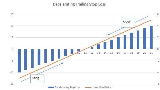
Image #11: Visualization of using a deceleration stop loss as gains are realized
One more advanced technique is the concept of Decelerating Stop Loss. Mostly used for intra-day models by which you want to preserve the returns you have gained thus far but still allow a runner to continue and accumulate returns.
The idea is to reduce your stop loss levels gradually as your returns are further cemented until you ultimately exit by hitting a trailing stop loss but at a much lower threshold compared to when the trade was started. This approach will take the trailing stop loss to a new level as the trailer still adjusts when a new high is reached (or a new low if you are targeting a short trade) but will also contract the stop limit accordingly.
Deep Reinforcement Learning for Exit Conditions
Reinforcement learning is a subset of machine learning in which an agent learns an optimal policy for interacting in its environment. A policy is a mapping from the state of an agent’s environment to actions. In the case of learning optimal bounds for exiting a position, environment is represented by a vector of features related to an asset. Actions, on the other hand, are represented by where bounds should be set as a function of ATR.

Image #12: Example of how reinforcement learning determines policy mapping features to actions.
Why use reinforcement learning? What makes it a good tool for financial data science? In recent years, reinforcement learning projects have made incredible strides in game playing. Google’s DeepMind created AlphaZero and AlphaGo – AIs that dominated humans and machines in chess and Go respectively. At the same time, Elon Musk’s nonprofit OpenAI created OpenAI Five – an AI that has beaten professional teams in the popular video game Dota 2.
Reinforcement learning’s appeal stems from the fact that it is a technique in which an agent learns directly from an environment. Just like the changing landscape of a game board, the stock market is an environment that is constantly in flux – multiple agents (investors) jockey to maximize reward (profits) employing a range of differing, constantly evolving, and sometimes adversarial strategies. Because reinforcement learning can adjust to the changing behavior of an environment, it is uniquely suited for learning optimal exit conditions.
At a high level, reinforcement learning functions by iteratively improving an agent’s policy according to the reward reaped from its actions. As such, effective learning is contingent upon having a well specified reward function. A reward function that is in some way deficient, for example being non-robust against noise, can easily create aberrant behavior.

Image #13: Examples of good and bad behaviors resulting from reinforcement learning.
Consider the “Undesirable Results” case at the top of Image #13 above. In this situation, the reinforcement learning agent has learned to produce exceedingly large threshold values. This is likely due to the fact that the agent learned from a period (in green) during which price experienced a great deal of volatility. Additionally, the reward reaped during the learning period was large and negative. As a result, the agent erroneously prefers extreme exit conditions that make realizing the loss unlikely. Such bounds are disadvantageous because they do not actually protect against losses. Furthermore, reaching such bounds would require significant price movements far beyond what is normal.
Conversely, consider the “Too Limited” case on Image #13. In this situation the opposite occurs. The agent produces very narrow thresholds because it learned over a short period of low volatility and was positively rewarded. Such narrow thresholds limit an investor’s profitable price action range. Additionally, by being easier to reach, the exit conditions are at increased risk of executing erroneously due to normal price volatility.
Both the “Better” and “Optimal Results” cases in Image #13 show how an agent might behave if it has learned properly. In these situations, the agent has balanced reward well and shows relative robustness to price volatility. Instead of setting bounds that are disproportionately large or narrow, it produces thresholds that are just right.
Reinforcement learning has appealing theoretical properties. An agent learns directly from data to choose exit thresholds that maximize a user-specified reward. This process is completely data-driven, thereby saving an investor from emotional exposure or from choosing an arbitrary ATR cut off at which to exit positions. Arbitrarily chosen ATR cut offs are almost certainly suboptimal – they can cause an investor to leave money “on the table” when tighter bounds are chosen, or endure unnecessary risk when looser ones are selected.


